as an ontological category reflects the measure of the possibility of the emergence of any entity in any conditions. In contrast to the mathematical and logical interpretations of this concept, ontological V. does not associate itself with the necessity of a quantitative expression. The value of V. is revealed in the context of understanding determinism and the nature of development in general.

Great Definition

Incomplete definition ↓

PROBABILITY

a concept that characterizes quantities. a measure of the possibility of the appearance of a certain event at a certain. conditions. In scientific knowledge there are three interpretations of V. The classical concept of V., which arose from the mathematical. analysis of gambling and most fully developed by B. Pascal, J. Bernoulli and P. Laplace, considers V. as the ratio of the number of favorable cases to the total number of all equally possible. For example, when throwing a die that has 6 sides, each of them can be expected to come up with a V equal to 1/6, since neither side has advantages over the other. Such symmetry of the outcomes of experience is specially taken into account when organizing games, but is relatively rare in the study of objective events in science and practice. Classic V.'s interpretation gave way to statistical. V.'s concepts, at the heart of which are valid. observation of the appearance of a certain event during the duration. experience under precisely fixed conditions. Practice confirms that the more often an event occurs, the greater the degree of the objective possibility of its occurrence, or V. Therefore, the statistical. V.'s interpretation is based on the concept of relates. frequencies, a cut can be determined empirically. V. as theoretical. the concept never coincides with an empirically determined frequency, however, in many ways. cases, it practically differs little from the relative. frequency found as a result of the duration. observations. Many statisticians regard V. as a "double" refers. frequency, edge is determined by statistical. study of observational results

or experiments. Less realistic was the definition of V. as the limit relates. frequencies of mass events, or collectives, proposed by R. Mises. As a further development of the frequency approach to V., a dispositional, or propensity, interpretation of V. is put forward (K. Popper, J. Hecking, M. Bunge, T. Setl). According to this interpretation, V. characterizes the property of generating conditions, for example. experiment. installation, to obtain a sequence of massive random events. It is this attitude that gives rise to the physical dispositions, or predispositions, V. to-rykh can be checked by means of relative. frequencies.

Statistical V.'s interpretation dominates the scientific. knowledge, because it reflects the specific. the nature of the patterns inherent in mass phenomena of a random nature. In many physical, biological, economic, demographic and other social processes, it is necessary to take into account the action of many random factors, to-rye are characterized by a stable frequency. Identification of this stable frequency and quantities. its assessment with the help of V. makes it possible to reveal the necessity, which makes its way through the cumulative action of many accidents. This is where the dialectic of the transformation of chance into necessity finds its manifestation (see F. Engels, in the book: K. Marx and F. Engels, Soch., vol. 20, pp. 535-36).

Logical or inductive reasoning characterizes the relationship between the premises and the conclusion of non-demonstrative and, in particular, inductive reasoning. Unlike deduction, the premises of induction do not guarantee the truth of the conclusion, but only make it more or less plausible. This credibility, with precisely formulated premises, can sometimes be estimated with the help of V. The value of this V. is most often determined by comparing. concepts (greater than, less than or equal to), and sometimes in a numerical way. Logic interpretation is often used to analyze inductive reasoning and build various systems of probabilistic logics (R. Carnap, R. Jeffrey). In the semantic logical concepts. V. is often defined as the degree of confirmation of one statement by others (for example, the hypothesis of its empirical data).

In connection with the development of theories of decision-making and games, the so-called. personalistic interpretation of V. Although V. in this case expresses the degree of faith of the subject and the occurrence of a certain event, V. themselves must be chosen in such a way that the axioms of the calculation of V. are satisfied. Therefore, V., with such an interpretation, expresses not so much the degree of subjective as rational faith . Consequently, decisions made on the basis of such V. will be rational, because they do not take into account the psychological. characteristics and inclinations of the subject.

From epistemological t. sp. difference between statistic., logical. and personalistic interpretations of V. lies in the fact that if the first characterizes the objective properties and relations of mass phenomena of a random nature, then the last two analyze the features of the subjective, cognizant. human activities under conditions of uncertainty.

PROBABILITY

one of the most important concepts of science, characterizing a special systemic vision of the world, its structure, evolution and cognition. The specificity of the probabilistic view of the world is revealed through the inclusion of the concepts of chance, independence and hierarchy (ideas of levels in the structure and determination of systems) among the basic concepts of being.

Ideas about probability originated in antiquity and were related to the characteristics of our knowledge, while the presence of probabilistic knowledge was recognized, which differs from reliable knowledge and from false. The impact of the idea of ​​probability on scientific thinking, on the development of knowledge is directly related to the development of the theory of probability as a mathematical discipline. The origin of the mathematical doctrine of probability dates back to the 17th century, when the development of the core of concepts that allow. quantitative (numerical) characteristics and expressing a probabilistic idea.

Intensive applications of probability to the development of knowledge fall on the 2nd floor. 19- 1st floor. 20th century Probability has entered the structures of such fundamental sciences of nature as classical statistical physics, genetics, quantum theory, cybernetics (information theory). Accordingly, probability personifies that stage in the development of science, which is now defined as non-classical science. To reveal the novelty, features of the probabilistic way of thinking, it is necessary to proceed from the analysis of the subject of probability theory and the foundations of its many applications. Probability theory is usually defined as a mathematical discipline that studies the laws of mass random phenomena under certain conditions. Randomness means that within the framework of mass character, the existence of each elementary phenomenon does not depend on and is not determined by the existence of other phenomena. At the same time, the very mass nature of phenomena has a stable structure, contains certain regularities. A mass phenomenon is quite strictly divided into subsystems, and the relative number of elementary phenomena in each of the subsystems (relative frequency) is very stable. This stability is compared with probability. A mass phenomenon as a whole is characterized by a distribution of probabilities, i.e., the assignment of subsystems and their corresponding probabilities. The language of probability theory is the language of probability distributions. Accordingly, the theory of probability is defined as the abstract science of operating with distributions.

Probability gave rise in science to ideas about statistical regularities and statistical systems. The latter are systems formed from independent or quasi-independent entities, their structure is characterized by probability distributions. But how is it possible to form systems from independent entities? It is usually assumed that for the formation of systems with integral characteristics, it is necessary that between their elements there are sufficiently stable bonds that cement the systems. The stability of statistical systems is given by the presence of external conditions, the external environment, external rather than internal forces. The very definition of probability is always based on setting the conditions for the formation of the initial mass phenomenon. Another important idea that characterizes the probabilistic paradigm is the idea of ​​hierarchy (subordination). This idea expresses the relationship between the characteristics of individual elements and the integral characteristics of systems: the latter, as it were, are built on top of the former.

The significance of probabilistic methods in cognition lies in the fact that they allow us to explore and theoretically express the patterns of structure and behavior of objects and systems that have a hierarchical, "two-level" structure.

Analysis of the nature of probability is based on its frequency, statistical interpretation. At the same time, for a very long time, such an understanding of probability dominated in science, which was called logical, or inductive, probability. Logical probability is interested in questions of the validity of a separate, individual judgment under certain conditions. Is it possible to assess the degree of confirmation (reliability, truth) of an inductive conclusion (hypothetical conclusion) in a quantitative form? In the course of the formation of the theory of probability, such questions were repeatedly discussed, and they began to talk about the degrees of confirmation of hypothetical conclusions. This measure of probability is determined by the information at the disposal of a given person, his experience, views on the world and the psychological mindset. In all such cases, the magnitude of the probability is not amenable to strict measurements and practically lies outside the competence of probability theory as a consistent mathematical discipline.

An objective, frequency interpretation of probability was established in science with considerable difficulty. Initially, the understanding of the nature of probability was strongly influenced by those philosophical and methodological views that were characteristic of classical science. Historically, the formation of probabilistic methods in physics occurred under the decisive influence of the ideas of mechanics: statistical systems were treated simply as mechanical ones. Since the corresponding problems were not solved by strict methods of mechanics, statements arose that the appeal to probabilistic methods and statistical regularities is the result of the incompleteness of our knowledge. In the history of the development of classical statistical physics, numerous attempts have been made to substantiate it on the basis of classical mechanics, but they all failed. The basis of probability is that it expresses the features of the structure of a certain class of systems, other than the systems of mechanics: the state of the elements of these systems is characterized by instability and a special (not reducible to mechanics) nature of interactions.

The entry of probability into cognition leads to the denial of the concept of rigid determinism, to the denial of the basic model of being and cognition developed in the process of the formation of classical science. The basic models represented by statistical theories are of a different, more general nature: they include the ideas of randomness and independence. The idea of ​​probability is connected with the disclosure of the internal dynamics of objects and systems, which cannot be completely determined by external conditions and circumstances.

The concept of a probabilistic vision of the world, based on the absolutization of ideas about independence (as before, the paradigm of rigid determination), has now revealed its limitations, which most strongly affects the transition of modern science to analytical methods for studying complex systems and the physical and mathematical foundations of self-organization phenomena.

Great Definition

Incomplete definition ↓

Probability of the opposite event

Consider some random event A, and let its probability p(A) known. Then the probability of the opposite event is determined by the formula

. (1.8)

Proof. Recall that according to axiom 3 for incompatible events

p(A+B) = p(A) + p(B).

Due to the incompatibility A And

Consequence., that is, the probability of an impossible event is zero.

Formula (1.8) is used to determine, for example, the probability of missing if the probability of hitting is known (or, conversely, the probability of hitting if the probability of missing is known; for example, if the probability of hitting for a gun is 0.9, the probability of a miss for it is (1 - 0, 9 = 0.1).

1. Probability of the sum of two events

Here it would be appropriate to recall that for incompatible events this formula looks like:

Example. The plant produces 85% of the products of the first grade and 10% of the second. The rest of the items are considered defective. What is the probability that, taking a product at random, we will get a defect?

Solution. P \u003d 1 - (0.85 + 0.1) \u003d 0.05.

The probability of the sum of any two random events is equal to

Proof. Imagine an event A + B as a sum of incompatible events

Given the incompatibility A and , we obtain according to Axiom 3

Similarly, we find

Substituting the latter into the previous formula, we obtain the desired (1.10) (Fig. 2).

Example. Of the 20 students, 5 people passed the exam in history for a deuce, 4 in English, and 3 students received deuces in both subjects. What is the percentage of students in the group who do not have twos in these subjects?

Solution. P = 1 - (5/20 + 4/20 - 3/20) = 0.7 (70%).

1. Conditional Probability

In some cases, it is necessary to determine the probability of a random event B assuming a random event has occurred A, which has a non-zero probability. That the event A happened, narrows the space of elementary events to a set A corresponding to this event. Further reasoning will be carried out on the example of a classical scheme. Let Wconsist of n equally possible elementary events (outcomes) and the event A favors m(A), and the event AB - m(AB) outcomes. Denote the conditional probability of an event B provided that A happened, - p(B|A). A-priory,

= .

If A happened, then one of the m(A) outcomes and event B can only happen if one of the favorable outcomes occurs AB; such outcomes m(AB). Therefore, it is natural to put the conditional probability of the event B provided that A happened, equal to the ratio

Summarizing, we give a general definition: conditional probability of event B, provided that event A with non-zero probability occurred , called

. (1.11)

It is easy to check that the definition introduced in this way satisfies all the axioms and, therefore, all previously proved theorems are true.

Often the conditional probability p(B|A) can be easily found from the conditions of the problem, in more complex cases one has to use definition (1.11).

Example. An urn contains N balls, of which n are white and N-n are black. A ball is taken out of it and, without putting it back ( sample without return ), get another one. What is the probability that both balls are white?

Solution. When solving this problem, we apply both the classical definition of probability and the product rule: we denote by A the event consisting in the fact that the white ball was taken out first (then the black ball was taken out first), and through B the event consisting in the fact that the second ball was taken out white ball; Then

.

It is easy to see that the probability that three balls taken out in a row (without replacement) are white is:

etc.

Example. Of the 30 examination cards, the student prepared only 25. If he refuses to answer the first ticket taken (which he does not know), then he is allowed to take the second one. Determine the probability that the second ticket is lucky.

Solution. Let the event A lies in the fact that the first ticket drawn turned out to be “bad” for the student, and B- the second - ²good ​​². Because after the event A one of the "bad" ones has already been extracted, then there are only 29 tickets left, of which 25 the student knows. Hence, the desired probability, assuming that the appearance of any ticket is equally possible and they do not return back, is equal to .

1. Product probability

Relation (1.11), assuming that p(A) or p(B) are not equal to zero, can be written in the form

This ratio is called theorem on the probability of the product of two events , which can be generalized to any number of factors, for example, for three it has the form

Example. Under the conditions of the previous example, find the probability of successfully passing the exam, if for this the student must answer the first ticket or, without answering the first one, be sure to answer the second one.

Solution. Let the events A And B are that, respectively, the first and second tickets are "good". Then - the appearance of a "bad" ticket for the first time. The exam will be taken if an event occurs A or at the same time and B. That is, the desired event C - the successful passing of the exam - is expressed as follows: C = A+ .From here

Here we have taken advantage of the incompatibility A and, hence, the incompatibility A and , theorems on the probability of sum and product and the classical definition of probability when calculating p(A) And .

This problem can be solved even more simply if we use the theorem on the probability of the opposite event:

1. Independence of events

Random events A and Blet's callindependent, If

For independent events, it follows from (1.11) that ; the converse is also true.

Independence of eventsmeans that the occurrence of event A does not change the probability of occurrence of event B, that is, the conditional probability is equal to the unconditional .

Example. Let's consider the previous example with an urn containing N balls, of which n are white, but let's change the experience: having taken out a ball, we put it back and only then take out the next one ( fetch with return ).

A is the event that the white ball was drawn first, the event that the black ball was drawn first, and B is the event that the white ball was drawn second; Then

that is, in this case the events A and B are independent.

Thus, when sampling with a return, the events at the second drawing of the ball are independent of the events of the first drawing, but when sampling without replacement, this is not the case. However, for large N and n, these probabilities are very close to each other. This is used because sampling without replacement is sometimes performed (for example, in quality control, when testing an object leads to its destruction), and the calculations are carried out using formulas for sampling with replacement, which are simpler.

In practice, when calculating probabilities, the rule is often used, according to which from the physical independence of events follows their independence in the probabilistic sense .

Example. The probability that a person aged 60 will not die in the next year is 0.91. An insurance company insures the life of two people aged 60 for a year.

Probability that none of them will die: 0.91 × 0.91 = 0.8281.

Probability of both of them dying:

(1 – 0.91)×(1 – 0.91) = 0.09 × 0.09 = 0.0081.

Probability of dying at least one:

1 – 0.91 × 0.91 = 1 – 0,8281 = 0,1719.

Probability of dying one:

0.91 x 0.09 + 0.09 x 0.91 = 0.1638.

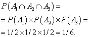
Event system A 1 , A 2 ,..., A n we call independent in the aggregate if the probability of the product is equal to the product of the probabilities for any combination of factors from this system. In this case, in particular,

Example. The code of the safe consists of seven decimal digits. What is the probability that the thief gets it right the first time?

In each of the 7 positions, you can dial any of the 10 digits 0,1,2,...,9, for a total of 10 7 numbers, starting from 0000000 and ending with 9999999.

Example. The code of the safe consists of a Russian letter (there are 33 of them) and three digits. What is the probability that the thief gets it right the first time?

P = (1/33) × (1/10) 3 .

Example. In a more general form, the insurance problem: the probability that a person aged ... years will not die in the next year is equal to p. An insurance company insures the life of n people of this age for a year.

The probability that no one of them will not die: pn (do not have to pay an insurance premium to anyone).

Probability of dying at least one: 1 - p n (payments are coming).

The likelihood that they All die: (1 – p) n (largest payouts).

Probability of dying one: n × (1 – p) × p n-1 (if people are numbered, then the one who dies can be numbered 1, 2,…,n – these are n different events, each of which has a probability of (1 – p) × pn-1).

1. Total Probability Formula

Let the events H 1 , H 2 , ... , H n satisfy the conditions

If .

Such a collection is called full group of events.

Let's assume that we know the probabilities p(H i), p(A/H i). In this case, applicable total probability formula

. (1.14)

Proof. Let's use what H i(they are usually called hypotheses ) are pairwise inconsistent (hence, inconsistent and H i× A), and their sum is a certain event

This scheme takes place whenever we can talk about the division of the entire space of events into several, generally speaking, heterogeneous regions. In economics, this is the division of a country or area into regions of different sizes and different conditions, when the share of each region is known p(Hi) and the probability (share) of some parameter in each region (for example, the percentage of unemployed - it is different in each region) - p(A/Hi). The warehouse may contain products from three different factories, supplying different quantities of products with different percentages of defects, etc.

Example. Casting in pigs comes from two shops to the third: 70% from the first and 30% from the second. At the same time, the products of the first workshop have 10% of defects, and the second - 20%. Find the probability that one disc, taken at random, has a defect.

Solution: p(H 1) = 0.7; p(H 2) = 0.3; p(A/H 1) = 0.1; p(A/H2)=0.2;

P = 0.7 × 0.1 + 0.3 × 0.2 = 0.13 (on average, 13% of blanks in the third shop are defective).

A mathematical model can be, for example, as follows: there are several urns of different composition; in the first urn there are n 1 balls, of which m 1 are white, and so on. The total probability formula is used to find the probability, by choosing an urn at random, to get a white ball out of it.

Problems are solved in the same way in the general case.

Example. Let's go back to the example with the urn containing N balls, of which n are white. We get out of it (without return) two balls. What is the probability that the second ball is white?

Solution. H 1 - the first ball is white; p(H 1)=n/N;

H 2 - the first ball is black; p(H2)=(N-n)/N;

B - the second ball is white; p(B|H 1)=(n-1)/(N-1); p(B|H2)=n/(N-1);

The same model can be applied to solve the following problem: out of N tickets, the student learned only n. What is more profitable for him - to pull the ticket the very first or the second? It turns out that in any case it is with probability n/N will draw a good ticket and with probability ( N-n)/N- bad.

Example. Determine the probability that a traveler leaving point A will end up at point B if at a fork in the road he randomly chooses any road (except the return one). The road map is shown in fig. 1.3.

Solution. Let the traveler's arrival at points H 1 , H 2 , H 3 and H 4 be the corresponding hypotheses. Obviously, they form a complete group of events and, by the condition of the problem,

p(H 1) = p(H 2) = p(H 3) = p(H 4) = 0,25.

(All directions from A are equally possible for the traveler). According to the road scheme, the conditional probabilities of hitting B, provided that the traveler passed through H i , are equal to:

Applying the total probability formula, we get

1. Bayes formula

Let us assume that the conditions of the previous paragraph are satisfied and it is additionally known that the event A happened. Find the probability that the hypothesis was realized H k. By definition of conditional probability

. (1.15)

The resulting ratio is called Bayes formula. She lets on known
(before the experiment) a priori probabilities of hypotheses p(Hi) and conditional probabilities p(A|Hi) determine the conditional probability p(H k |A), which is called a posteriori (that is, obtained on the condition that, as a result of the experience, the event A already happened).

Example. 30% of patients admitted to the hospital belong to the first social group, 20% - to the second and 50% - to the third. The probability of contracting tuberculosis for a representative of each social group, respectively, is 0.02, 0.03 and 0.01. Tests performed for a randomly selected patient showed the presence of tuberculosis. Find the probability that this is a representative of the third group.

It is unlikely that many people think about whether it is possible to calculate events that are more or less random. In simple terms, is it realistic to know which side of the die will fall next. It was this question that two great scientists asked, who laid the foundation for such a science as the theory of probability, in which the probability of an event is studied quite extensively.

Origin

If you try to define such a concept as probability theory, you get the following: this is one of the branches of mathematics that studies the constancy of random events. Of course, this concept does not really reveal the whole essence, so it is necessary to consider it in more detail.

I would like to start with the creators of the theory. As mentioned above, there were two of them, and it was they who were among the first who tried to calculate the outcome of an event using formulas and mathematical calculations. On the whole, the beginnings of this science appeared in the Middle Ages. At that time, various thinkers and scientists tried to analyze gambling, such as roulette, dice, and so on, thereby establishing a pattern and percentage of a particular number falling out. The foundation was laid in the seventeenth century by the aforementioned scientists.

At first, their work could not be attributed to the great achievements in this field, because everything they did was simply empirical facts, and the experiments were made visually, without the use of formulas. Over time, it turned out to achieve great results, which appeared as a result of observing the throwing of dice. It was this tool that helped to derive the first intelligible formulas.

Like-minded people

It is impossible not to mention such a person as Christian Huygens, in the process of studying a topic called "probability theory" (the probability of an event is covered precisely in this science). This person is very interesting. He, like the scientists presented above, tried to derive the regularity of random events in the form of mathematical formulas. It is noteworthy that he did not do this together with Pascal and Fermat, that is, all his works did not in any way intersect with these minds. Huygens brought out

An interesting fact is that his work came out long before the results of the work of the discoverers, or rather, twenty years earlier. Among the designated concepts, the most famous are:

• the concept of probability as a magnitude of chance;
• mathematical expectation for discrete cases;
• theorems of multiplication and addition of probabilities.

It is also impossible not to remember who also made a significant contribution to the study of the problem. Conducting his own tests, independent of anyone, he managed to present a proof of the law of large numbers. In turn, the scientists Poisson and Laplace, who worked at the beginning of the nineteenth century, were able to prove the original theorems. It was from this moment that probability theory began to be used to analyze errors in the course of observations. Russian scientists, or rather Markov, Chebyshev and Dyapunov, could not bypass this science either. Based on the work done by the great geniuses, they fixed this subject as a branch of mathematics. These figures worked already at the end of the nineteenth century, and thanks to their contribution, phenomena such as:

• law of large numbers;
• theory of Markov chains;
• central limit theorem.

So, with the history of the birth of science and with the main people who influenced it, everything is more or less clear. Now it's time to concretize all the facts.

Basic concepts

Before touching on laws and theorems, it is worth studying the basic concepts of probability theory. The event takes the leading role in it. This topic is quite voluminous, but without it it will not be possible to understand everything else.

An event in probability theory is any set of outcomes of an experiment. There are not so many concepts of this phenomenon. So, the scientist Lotman, who works in this area, said that in this case we are talking about what "happened, although it might not have happened."

Random events (probability theory pays special attention to them) is a concept that implies absolutely any phenomenon that has the ability to occur. Or, conversely, this scenario may not happen when many conditions are met. It is also worth knowing that it is random events that capture the entire volume of phenomena that have occurred. Probability theory indicates that all conditions can be repeated constantly. It was their conduct that was called "experiment" or "test".

A certain event is one that will 100% occur in a given test. Accordingly, an impossible event is one that will not happen.

The combination of a pair of actions (conditionally case A and case B) is a phenomenon that occurs simultaneously. They are designated as AB.

The sum of pairs of events A and B is C, in other words, if at least one of them happens (A or B), then C will be obtained. The formula of the described phenomenon is written as follows: C \u003d A + B.

Disjoint events in probability theory imply that the two cases are mutually exclusive. They can never happen at the same time. Joint events in probability theory are their antipode. This implies that if A happened, then it does not prevent B in any way.

Opposite events (probability theory deals with them in great detail) are easy to understand. It is best to deal with them in comparison. They are almost the same as incompatible events in probability theory. But their difference lies in the fact that one of the many phenomena in any case must occur.

Equally probable events are those actions, the possibility of repetition of which is equal. To make it clearer, we can imagine the tossing of a coin: the loss of one of its sides is equally likely to fall out of the other.

A favorable event is easier to see with an example. Let's say there is episode B and episode A. The first is the roll of the die with the appearance of an odd number, and the second is the appearance of the number five on the die. Then it turns out that A favors B.

Independent events in the theory of probability are projected only on two or more cases and imply the independence of any action from another. For example, A - dropping tails when throwing a coin, and B - getting a jack from the deck. They are independent events in probability theory. At this point, it became clearer.

Dependent events in probability theory are also admissible only for their set. They imply the dependence of one on the other, that is, the phenomenon B can occur only if A has already happened or, on the contrary, has not happened when this is the main condition for B.

The outcome of a random experiment consisting of one component is elementary events. Probability theory explains that this is a phenomenon that happened only once.

Basic Formulas

So, the concepts of "event", "probability theory" were considered above, the definition of the main terms of this science was also given. Now it's time to get acquainted directly with the important formulas. These expressions mathematically confirm all the main concepts in such a difficult subject as probability theory. The probability of an event plays a huge role here too.

It is better to start with the main ones. And before proceeding to them, it is worth considering what it is.

Combinatorics is primarily a branch of mathematics, it deals with the study of a huge number of integers, as well as various permutations of both the numbers themselves and their elements, various data, etc., leading to the appearance of a number of combinations. In addition to probability theory, this branch is important for statistics, computer science, and cryptography.

So, now you can move on to the presentation of the formulas themselves and their definition.

The first of these will be an expression for the number of permutations, it looks like this:

P_n = n ⋅ (n - 1) ⋅ (n - 2)…3 ⋅ 2 ⋅ 1 = n!

The equation applies only if the elements differ only in their order.

Now the placement formula will be considered, it looks like this:

A_n^m = n ⋅ (n - 1) ⋅ (n-2) ⋅ ... ⋅ (n - m + 1) = n! : (n - m)!

This expression is applicable not only to the order of the element, but also to its composition.

The third equation from combinatorics, and it is also the last one, is called the formula for the number of combinations:

C_n^m = n ! : ((n - m))! :m!

A combination is called a selection that is not ordered, respectively, and this rule applies to them.

It turned out to be easy to figure out the formulas of combinatorics, now we can move on to the classical definition of probabilities. This expression looks like this:

In this formula, m is the number of conditions favorable to the event A, and n is the number of absolutely all equally possible and elementary outcomes.

There are a large number of expressions, the article will not cover all of them, but the most important of them will be touched upon, such as, for example, the probability of the sum of events:

P(A + B) = P(A) + P(B) - this theorem is for adding only incompatible events;

P(A + B) = P(A) + P(B) - P(AB) - and this one is for adding only compatible ones.

Probability of producing events:

P(A ⋅ B) = P(A) ⋅ P(B) - this theorem is for independent events;

(P(A ⋅ B) = P(A) ⋅ P(B∣A); P(A ⋅ B) = P(A) ⋅ P(A∣B)) - and this one is for dependents.

The event formula will end the list. Probability theory tells us about Bayes' theorem, which looks like this:

P(H_m∣A) = (P(H_m)P(A∣H_m)) : (∑_(k=1)^n P(H_k)P(A∣H_k)),m = 1,..., n

In this formula, H 1 , H 2 , …, H n is the full group of hypotheses.

Examples

If you carefully study any branch of mathematics, it is not complete without exercises and sample solutions. So is the theory of probability: events, examples here are an integral component that confirms scientific calculations.

Formula for number of permutations

Let's say there are thirty cards in a deck of cards, starting with face value one. Next question. How many ways are there to stack the deck so that cards with a face value of one and two are not next to each other?

The task is set, now let's move on to solving it. First you need to determine the number of permutations of thirty elements, for this we take the above formula, it turns out P_30 = 30!.

Based on this rule, we will find out how many options there are to fold the deck in different ways, but we need to subtract from them those in which the first and second cards are next. To do this, let's start with the option when the first is above the second. It turns out that the first card can take twenty-nine places - from the first to the twenty-ninth, and the second card from the second to the thirtieth, it turns out only twenty-nine places for a pair of cards. In turn, the rest can take twenty-eight places, and in any order. That is, for a permutation of twenty-eight cards, there are twenty-eight options P_28 = 28!

As a result, it turns out that if we consider the solution when the first card is above the second, there are 29 ⋅ 28 extra possibilities! = 29!

Using the same method, you need to calculate the number of redundant options for the case when the first card is under the second. It also turns out 29 ⋅ 28! = 29!

From this it follows that there are 2 ⋅ 29! extra options, while there are 30 necessary ways to build the deck! - 2 ⋅ 29!. It remains only to count.

30! = 29! ⋅ 30; 30!- 2 ⋅ 29! = 29! ⋅ (30 - 2) = 29! ⋅ 28

Now you need to multiply all the numbers from one to twenty-nine among themselves, and then at the end multiply everything by 28. The answer is 2.4757335 ⋅〖10〗^32

Example solution. Formula for Placement Number

In this problem, you need to find out how many ways there are to put fifteen volumes on one shelf, but on the condition that there are thirty volumes in total.

In this problem, the solution is slightly simpler than in the previous one. Using the already known formula, it is necessary to calculate the total number of arrangements from thirty volumes of fifteen.

A_30^15 = 30 ⋅ 29 ⋅ 28⋅... ⋅ (30 - 15 + 1) = 30 ⋅ 29 ⋅ 28 ⋅ ... ⋅ 16 = 202 843 204 931 727 360 000

The answer, respectively, will be equal to 202,843,204,931,727,360,000.

Now let's take the task a little more difficult. You need to find out how many ways there are to arrange thirty books on two bookshelves, provided that only fifteen volumes can be on one shelf.

Before starting the solution, I would like to clarify that some problems are solved in several ways, so there are two ways in this one, but the same formula is used in both.

In this problem, you can take the answer from the previous one, because there we calculated how many times you can fill a shelf with fifteen books in different ways. It turned out A_30^15 = 30 ⋅ 29 ⋅ 28 ⋅ ... ⋅ (30 - 15 + 1) = 30 ⋅ 29 ⋅ 28 ⋅ ...⋅ 16.

We calculate the second shelf according to the permutation formula, because fifteen books are placed in it, while only fifteen remain. We use the formula P_15 = 15!.

It turns out that in total there will be A_30^15 ⋅ P_15 ways, but, in addition, the product of all numbers from thirty to sixteen will need to be multiplied by the product of numbers from one to fifteen, as a result, the product of all numbers from one to thirty will be obtained, that is, the answer equals 30!

But this problem can be solved in a different way - easier. To do this, you can imagine that there is one shelf for thirty books. All of them are placed on this plane, but since the condition requires that there be two shelves, we cut one long one in half, it turns out two fifteen each. From this it turns out that the placement options can be P_30 = 30!.

Example solution. Formula for combination number

Now we will consider a variant of the third problem from combinatorics. You need to find out how many ways there are to arrange fifteen books, provided that you need to choose from thirty absolutely identical ones.

For the solution, of course, the formula for the number of combinations will be applied. From the condition it becomes clear that the order of the identical fifteen books is not important. Therefore, initially you need to find out the total number of combinations of thirty books of fifteen.

C_30^15 = 30 ! : ((30-15)) ! : 15 ! = 155 117 520

That's all. Using this formula, in the shortest possible time it was possible to solve such a problem, the answer, respectively, is 155 117 520.

Example solution. The classical definition of probability

Using the formula above, you can find the answer in a simple problem. But it will help to visually see and trace the course of actions.

The problem is given that there are ten absolutely identical balls in the urn. Of these, four are yellow and six are blue. One ball is taken from the urn. You need to find out the probability of getting blue.

To solve the problem, it is necessary to designate getting the blue ball as event A. This experience can have ten outcomes, which, in turn, are elementary and equally probable. At the same time, six out of ten are favorable for event A. We solve using the formula:

P(A) = 6: 10 = 0.6

By applying this formula, we found out that the probability of getting a blue ball is 0.6.

Example solution. Probability of the sum of events

Now a variant will be presented, which is solved using the formula for the probability of the sum of events. So, in the condition given that there are two boxes, the first contains one gray and five white balls, and the second contains eight gray and four white balls. As a result, one of them was taken from the first and second boxes. It is necessary to find out what is the chance that the balls taken out will be gray and white.

To solve this problem, it is necessary to designate events.

• So, A - take a gray ball from the first box: P(A) = 1/6.
• A '- they took a white ball also from the first box: P (A ") \u003d 5/6.
• B - a gray ball was taken out already from the second box: P(B) = 2/3.
• B' - they took a gray ball from the second box: P(B") = 1/3.

According to the condition of the problem, it is necessary that one of the phenomena occur: AB 'or A'B. Using the formula, we get: P(AB") = 1/18, P(A"B) = 10/18.

Now the formula for multiplying the probability has been used. Next, to find out the answer, you need to apply the equation for their addition:

P = P(AB" + A"B) = P(AB") + P(A"B) = 11/18.

So, using the formula, you can solve similar problems.

Outcome

The article provided information on the topic "Probability Theory", in which the probability of an event plays a crucial role. Of course, not everything was taken into account, but, based on the text presented, one can theoretically get acquainted with this section of mathematics. The science in question can be useful not only in professional work, but also in everyday life. With its help, you can calculate any possibility of any event.

The text also touched upon significant dates in the history of the formation of the theory of probability as a science, and the names of people whose works were invested in it. This is how human curiosity led to the fact that people learned to calculate even random events. Once they were just interested in it, but today everyone already knows about it. And no one will say what awaits us in the future, what other brilliant discoveries related to the theory under consideration will be made. But one thing is for sure - research does not stand still!

The need for operations on probabilities comes when the probabilities of some events are known, and it is necessary to calculate the probabilities of other events that are associated with these events.

Probability addition is used when it is necessary to calculate the probability of a combination or a logical sum of random events.

Sum of events A And B designate A + B or A ∪ B. The sum of two events is an event that occurs if and only if at least one of the events occurs. It means that A + B- an event that occurs if and only if an event occurs during the observation A or event B, or at the same time A And B.

If events A And B are mutually inconsistent and their probabilities are given, then the probability that one of these events will occur as a result of one trial is calculated using the addition of probabilities.

The theorem of addition of probabilities. The probability that one of two mutually incompatible events will occur is equal to the sum of the probabilities of these events:

For example, two shots were fired while hunting. Event A– hitting a duck from the first shot, event IN– hit from the second shot, event ( A+ IN) - hit from the first or second shot or from two shots. So if two events A And IN are incompatible events, then A+ IN- the occurrence of at least one of these events or two events.

Example 1 A box contains 30 balls of the same size: 10 red, 5 blue and 15 white. Calculate the probability that a colored (not white) ball is taken without looking.

Solution. Let's assume that the event A– “the red ball is taken”, and the event IN- "The blue ball is taken." Then the event is “a colored (not white) ball is taken”. Find the probability of an event A:

and events IN:

Events A And IN- mutually incompatible, since if one ball is taken, then balls of different colors cannot be taken. Therefore, we use the addition of probabilities:

The theorem of addition of probabilities for several incompatible events. If the events make up the complete set of events, then the sum of their probabilities is equal to 1:

The sum of the probabilities of opposite events is also equal to 1:

Opposite events form a complete set of events, and the probability of a complete set of events is 1.

The probabilities of opposite events are usually denoted in small letters. p And q. In particular,

from which the following formulas for the probability of opposite events follow:

Example 2 The target in the dash is divided into 3 zones. The probability that a certain shooter will shoot at a target in the first zone is 0.15, in the second zone - 0.23, in the third zone - 0.17. Find the probability that the shooter hits the target and the probability that the shooter misses the target.

Solution: Find the probability that the shooter hits the target:

Find the probability that the shooter misses the target:

More difficult tasks in which you need to apply both addition and multiplication of probabilities - on the page "Various tasks for addition and multiplication of probabilities" .

Addition of probabilities of mutually joint events

Two random events are said to be joint if the occurrence of one event does not preclude the occurrence of a second event in the same observation. For example, when throwing a dice, the event A is considered to be the occurrence of the number 4, and the event IN- dropping an even number. Since the number 4 is an even number, the two events are compatible. In practice, there are tasks for calculating the probabilities of the occurrence of one of the mutually joint events.

The theorem of addition of probabilities for joint events. The probability that one of the joint events will occur is equal to the sum of the probabilities of these events, from which the probability of the common occurrence of both events is subtracted, that is, the product of the probabilities. The formula for the probabilities of joint events is as follows:

Because the events A And IN compatible, event A+ IN occurs if one of three possible events occurs: or AB. According to the theorem of addition of incompatible events, we calculate as follows:

Event A occurs if one of two incompatible events occurs: or AB. However, the probability of occurrence of one event from several incompatible events is equal to the sum of the probabilities of all these events:

Similarly:

Substituting expressions (6) and (7) into expression (5), we obtain the probability formula for joint events:

When using formula (8), it should be taken into account that the events A And IN can be:

• mutually independent;
• mutually dependent.

Probability formula for mutually independent events:

Probability formula for mutually dependent events:

If events A And IN are inconsistent, then their coincidence is an impossible case and, thus, P(AB) = 0. The fourth probability formula for incompatible events is as follows:

Example 3 In auto racing, when driving in the first car, the probability of winning, when driving in the second car. Find:

• the probability that both cars will win;
• the probability that at least one car will win;

1) The probability that the first car will win does not depend on the result of the second car, so the events A(first car wins) and IN(second car wins) - independent events. Find the probability that both cars win:

2) Find the probability that one of the two cars will win:

More difficult tasks in which you need to apply both addition and multiplication of probabilities - on the page "Various tasks for addition and multiplication of probabilities" .

Solve the problem of addition of probabilities yourself, and then look at the solution

Example 4 Two coins are thrown. Event A- loss of coat of arms on the first coin. Event B- loss of coat of arms on the second coin. Find the probability of an event C = A + B .

Probability multiplication

Multiplication of probabilities is used when the probability of a logical product of events is to be calculated.

In this case, random events must be independent. Two events are said to be mutually independent if the occurrence of one event does not affect the probability of the occurrence of the second event.

Probability multiplication theorem for independent events. The probability of the simultaneous occurrence of two independent events A And IN is equal to the product of the probabilities of these events and is calculated by the formula:

Example 5 The coin is tossed three times in a row. Find the probability that the coat of arms will fall out all three times.

Solution. The probability that the coat of arms will fall on the first toss of a coin, the second time, and the third time. Find the probability that the coat of arms will fall out all three times:

Solve problems for multiplying probabilities yourself, and then look at the solution

Example 6 There is a box with nine new tennis balls. Three balls are taken for the game, after the game they are put back. When choosing balls, they do not distinguish between played and unplayed balls. What is the probability that after three games there will be no unplayed balls in the box?

Example 7 32 letters of the Russian alphabet are written on cut alphabet cards. Five cards are drawn at random, one after the other, and placed on the table in the order in which they appear. Find the probability that the letters will form the word "end".

Example 8 From a full deck of cards (52 sheets), four cards are taken out at once. Find the probability that all four of these cards are of the same suit.

Example 9 The same problem as in example 8, but each card is returned to the deck after being drawn.

More complex tasks, in which you need to apply both addition and multiplication of probabilities, as well as calculate the product of several events, on the page "Various tasks for addition and multiplication of probabilities" .

The probability that at least one of the mutually independent events will occur can be calculated by subtracting the product of the probabilities of opposite events from 1, that is, by the formula:

Example 10 Cargoes are delivered by three modes of transport: river, rail and road transport. The probability that the cargo will be delivered by river transport is 0.82, by rail 0.87, by road 0.90. Find the probability that the goods will be delivered by at least one of the three modes of transport.

When a coin is tossed, it can be said that it will land heads up, or probability of this is 1/2. Of course, this does not mean that if a coin is tossed 10 times, it will necessarily land on heads 5 times. If the coin is "fair" and if it is tossed many times, then heads will come up very close half the time. Thus, there are two kinds of probabilities: experimental And theoretical .

Experimental and theoretical probability

If we toss a coin a large number of times - say 1000 - and count how many times it comes up heads, we can determine the probability that it will come up heads. If heads come up 503 times, we can calculate the probability of it coming up:
503/1000, or 0.503.

This experimental definition of probability. This definition of probability stems from observation and study of data and is quite common and very useful. For example, here are some probabilities that were determined experimentally:

1. The chance of a woman developing breast cancer is 1/11.

2. If you kiss someone who has a cold, then the probability that you will also get a cold is 0.07.

3. A person who has just been released from prison has an 80% chance of going back to prison.

If we consider the toss of a coin and taking into account that it is equally likely to come up heads or tails, we can calculate the probability of coming up heads: 1 / 2. This is the theoretical definition of probability. Here are some other probabilities that have been theoretically determined using mathematics:

1. If there are 30 people in a room, the probability that two of them have the same birthday (excluding the year) is 0.706.

2. During a trip, you meet someone and during the course of the conversation you discover that you have a mutual acquaintance. Typical reaction: "That can't be!" In fact, this phrase does not fit, because the probability of such an event is quite high - just over 22%.

Therefore, the experimental probability is determined by observation and data collection. Theoretical probabilities are determined by mathematical reasoning. Examples of experimental and theoretical probabilities, such as those discussed above, and especially those that we do not expect, lead us to the importance of studying probability. You may ask, "What is true probability?" Actually, there is none. It is experimentally possible to determine the probabilities within certain limits. They may or may not coincide with the probabilities that we obtain theoretically. There are situations in which it is much easier to define one type of probability than another. For example, it would be sufficient to find the probability of catching a cold using theoretical probability.

Calculation of experimental probabilities

Consider first the experimental definition of probability. The basic principle we use to calculate such probabilities is as follows.

Principle P (experimental)

If in an experiment in which n observations are made, the situation or event E occurs m times in n observations, then the experimental probability of the event is said to be P (E) = m/n.

Example 1 Sociological survey. An experimental study was conducted to determine the number of left-handers, right-handers and people in whom both hands are equally developed. The results are shown in the graph.

a) Determine the probability that the person is right-handed.

b) Determine the probability that the person is left-handed.

c) Determine the probability that the person is equally fluent in both hands.

d) Most PBA tournaments have 120 players. Based on this experiment, how many players can be left-handed?

Solution

a) The number of people who are right-handed is 82, the number of left-handers is 17, and the number of those who are equally fluent in both hands is 1. The total number of observations is 100. Thus, the probability that a person is right-handed is P
P = 82/100, or 0.82, or 82%.

b) The probability that a person is left-handed is P, where
P = 17/100 or 0.17 or 17%.

c) The probability that a person is equally fluent with both hands is P, where
P = 1/100 or 0.01 or 1%.

d) 120 bowlers and from (b) we can expect 17% to be left handed. From here
17% of 120 = 0.17.120 = 20.4,
that is, we can expect about 20 players to be left-handed.

Example 2 Quality control . It is very important for a manufacturer to keep the quality of their products at a high level. In fact, companies hire quality control inspectors to ensure this process. The goal is to release the minimum possible number of defective products. But since the company produces thousands of items every day, it cannot afford to inspect each item to determine if it is defective or not. To find out what percentage of products are defective, the company tests far fewer products.
The USDA requires that 80% of the seeds that growers sell germinate. To determine the quality of the seeds that the agricultural company produces, 500 seeds are planted from those that have been produced. After that, it was calculated that 417 seeds germinated.

a) What is the probability that the seed will germinate?

b) Do the seeds meet government standards?

Solution a) We know that out of 500 seeds that were planted, 417 sprouted. The probability of seed germination P, and
P = 417/500 = 0.834, or 83.4%.

b) Since the percentage of germinated seeds exceeded 80% on demand, the seeds meet the state standards.

Example 3 TV ratings. According to statistics, there are 105,500,000 TV households in the United States. Every week, information about viewing programs is collected and processed. Within one week, 7,815,000 households were tuned in to CBS' hit comedy series Everybody Loves Raymond and 8,302,000 households were tuned in to NBC's hit Law & Order (Source: Nielsen Media Research). What is the probability that one home's TV is tuned to "Everybody Loves Raymond" during a given week? to "Law & Order"?

Solution The probability that the TV in one household is set to "Everybody Loves Raymond" is P, and
P = 7.815.000/105.500.000 ≈ 0.074 ≈ 7.4%.
The possibility that the household TV was set to "Law & Order" is P, and
P = 8.302.000/105.500.000 ≈ 0.079 ≈ 7.9%.
These percentages are called ratings.

theoretical probability

Suppose we are doing an experiment, such as tossing a coin or dart, drawing a card from a deck, or testing items on an assembly line. Each possible outcome of such an experiment is called Exodus . The set of all possible outcomes is called outcome space . Event it is a set of outcomes, that is, a subset of the space of outcomes.

Example 4 Throwing darts. Suppose that in the "throwing darts" experiment, the dart hits the target. Find each of the following:

b) Outcome space

Solution
a) Outcomes are: hitting black (H), hitting red (K) and hitting white (B).

b) There is an outcome space (hit black, hit red, hit white), which can be written simply as (B, R, B).

Example 5 Throwing dice. A die is a cube with six sides, each of which has one to six dots.


Suppose we are throwing a die. Find
a) Outcomes
b) Outcome space

Solution
a) Outcomes: 1, 2, 3, 4, 5, 6.
b) Outcome space (1, 2, 3, 4, 5, 6).

We denote the probability that an event E occurs as P(E). For example, "the coin will land on tails" can be denoted by H. Then P(H) is the probability that the coin will land on tails. When all outcomes of an experiment have the same probability of occurring, they are said to be equally likely. To see the difference between events that are equally likely and events that are not equally likely, consider the target shown below.

For target A, black, red, and white hit events are equally likely, since black, red, and white sectors are the same. However, for target B, the zones with these colors are not the same, that is, hitting them is not equally likely.

Principle P (Theoretical)

If an event E can happen in m ways out of n possible equiprobable outcomes from the outcome space S, then theoretical probability event, P(E) is
P(E) = m/n.

Example 6 What is the probability of rolling a 3 by rolling a die?

Solution There are 6 equally likely outcomes on the die and there is only one possibility of throwing the number 3. Then the probability P will be P(3) = 1/6.

Example 7 What is the probability of rolling an even number on the die?

Solution The event is the throwing of an even number. This can happen in 3 ways (if you roll 2, 4 or 6). The number of equiprobable outcomes is 6. Then the probability P(even) = 3/6, or 1/2.

We will be using a number of examples related to a standard 52-card deck. Such a deck consists of the cards shown in the figure below.

Example 8 What is the probability of drawing an ace from a well-shuffled deck of cards?

Solution There are 52 outcomes (the number of cards in the deck), they are equally likely (if the deck is well mixed), and there are 4 ways to draw an ace, so according to the P principle, the probability
P(drawing an ace) = 4/52, or 1/13.

Example 9 Suppose we choose without looking one marble from a bag of 3 red marbles and 4 green marbles. What is the probability of choosing a red ball?

Solution There are 7 equally likely outcomes to get any ball, and since the number of ways to draw a red ball is 3, we get
P(choosing a red ball) = 3/7.

The following statements are results from the P principle.

Probability Properties

a) If the event E cannot happen, then P(E) = 0.
b) If the event E is bound to happen then P(E) = 1.
c) The probability that event E will occur is a number between 0 and 1: 0 ≤ P(E) ≤ 1.

For example, in tossing a coin, the event that the coin lands on its edge has zero probability. The probability that a coin is either heads or tails has a probability of 1.

Example 10 Suppose that 2 cards are drawn from a deck with 52 cards. What is the probability that both of them are spades?

Solution The number of ways n of drawing 2 cards from a well-shuffled 52-card deck is 52 C 2 . Since 13 of the 52 cards are spades, the number m of ways to draw 2 spades is 13 C 2 . Then,
P(stretching 2 peaks) \u003d m / n \u003d 13 C 2 / 52 C 2 \u003d 78/1326 \u003d 1/17.

Example 11 Suppose 3 people are randomly selected from a group of 6 men and 4 women. What is the probability that 1 man and 2 women will be chosen?

Solution Number of ways to choose three people from a group of 10 people 10 C 3 . One man can be chosen in 6 C 1 ways and 2 women can be chosen in 4 C 2 ways. According to the fundamental principle of counting, the number of ways to choose the 1st man and 2 women is 6 C 1 . 4C2. Then, the probability that 1 man and 2 women will be chosen is
P = 6 C 1 . 4 C 2 / 10 C 3 \u003d 3/10.

Example 12 Throwing dice. What is the probability of throwing a total of 8 on two dice?

Solution There are 6 possible outcomes on each dice. The outcomes are doubled, that is, there are 6.6 or 36 possible ways in which the numbers on two dice can fall. (It's better if the cubes are different, say one is red and the other is blue - this will help visualize the result.)

Pairs of numbers that add up to 8 are shown in the figure below. There are 5 possible ways to get the sum equal to 8, hence the probability is 5/36.