Consider algorithms for modeling the stationary normal and Markov random processes. These processes are widely used as mathematical models of various kinds of real processes occurring in complex technical systems. Below, we give some definitions and concepts that are essential for further presentation and are accepted in the framework of the correlation and spectral theories. random functions.
random function is called a function of a non-random argument t, which, for each fixed value of the argument, is a random variable. random function time called random process. random function coordinates points in space are called random field. The specific form taken by a random process as a result of experience is called the realization (trajectory) of a random process. All obtained implementations of the random process constitute an ensemble of implementations. The values of realizations at specific moments of time (time sections) are called instantaneous values of a random process.
We introduce the following notation: X(t) - random process; x i (t) - i-th implementation of the process X(t); x i (t j) - instantaneous value of the process Х(t), corresponding to the i-th realization at the j-th moment of time. The set of instantaneous values corresponding to the values of different implementations at the same time t j , we call the j-th sequence of the process X(t) and denote x(t j). From what has been said, it follows that time and implementation number can act as arguments of a random process. In this regard, two approaches to studying the properties of a random process are legitimate: the first is based on the analysis of a set of realizations, the second operates with a set of sequences - time sections. The presence or absence of dependence of the values of the probabilistic characteristics of a random process on time or the implementation number determines such fundamental properties of the process as stationarity and ergodicity. Stationary is a process whose probabilistic characteristics do not depend on time. Ergodic a process is called, the probabilistic characteristics of which do not depend on the implementation number.
The random process is called normal(or Gaussian) process, if the one-dimensional and two-dimensional distribution laws of any of its sections are normal. The exhaustive characteristics of a normal random process are its mathematical expectation and correlation function. For a stationary normal random process, the IOL is constant, and the correlation function depends only on the difference in time points for which the ordinates of the random process are taken ( =t 2 -t 1). For a stationary random process with a sufficiently large deviation of the ordinate of the random process X (t 2) from its mathematical expectation m x at time t 2 becomes practically independent of the value of this deviation at time t 1 . In this case, the correlation function K(t), which gives the value of the moment of connection between X(t 2) and X(t 1), at will tend to zero. Therefore, K () can either decrease monotonically, as shown in Fig. 2.2, or have the form shown in Fig. 2.3. The function of the form (Fig. 2.2.), as a rule, is approximated by the expressions:
![]() (2.38)
(2.38)
and the function of the form (Fig. 2.3.) - by expressions:

Fig.2.2. Fig.2.3.
The stability of a stationary random process in time makes it possible to replace the argument - time - with some auxiliary variable, which in many applications has the dimension of frequency. This substitution makes it possible to significantly simplify the calculations and achieve greater clarity of the results. The resulting function (S()) is called the spectral density of a stationary random process and is related to the correlation function by mutually inverse Fourier transforms:
![]() (2.42)
(2.42)
![]() (2.43)
(2.43)
There are other normalizations of the spectral density, for example:
![]() (2.44)
(2.44)
Based on the Fourier transforms, it is easy to obtain, for example, for a random process with K(t) of the form (2.38):
![]() (2.45)
(2.45)
A stationary random process whose spectral density is constant (S(w)=S=const) is called stationary white noise. The correlation function of stationary white noise is equal to zero for all , which means that any two of its sections are not correlated.
The problem of modeling a stationary normal random process (SNSP) can be formulated as the problem of finding an algorithm that makes it possible to obtain discrete implementations of this process on a computer. The process X(t) is replaced with a given accuracy by the corresponding process X(nDt) with discrete time t n = nDt (Dt is the sampling step of the process, n is an integer argument). As a result, the random process x(t) will be assigned random sequences:
x k [n]=x k (nDt), (2.46)
where k is the implementation number.
Obviously, an arbitrary member of the random sequence x(nDt) can be considered as a random function of its number, i.e. integer argument n and thus exclude Dt from consideration, which is taken into account when writing (2.46). In addition, to distinguish an integer argument from a continuously varying argument, it is enclosed in square brackets.
Random sequences are often referred to as discrete random processes or time series.
It is known that adding a non-random variable to a random function does not change the value of the correlation function. Therefore, in practice, centered stochastic processes are very often modeled (MOF is equal to zero), from which one can always go to real way adding MU to the members of a random sequence simulating a random process.
For random sequences, the correlation function and spectral density are calculated from the dependencies:
 (2.47)
![]() (2.48)
(2.48)
Reducing a random process to a random sequence essentially means replacing it with a multidimensional vector. Therefore, the considered method of modeling random vectors, generally speaking, is suitable for modeling random processes given on a finite time interval. However, for stationary normal random processes, there are more effective methods construction of modeling algorithms. Let's consider two methods that greatest application on practice.
1. L. P. Akimov, Yu. M. Gorodetsky, and S. I. Shukuryan, “On the modeling of Gaussian random sequences on digital computers,” Zh. "Automation and telemechanics", 1969, No. 1.
2. P. A. Bakut, I. A. Bol’shakov, et al., Questions of the Statistical Theory of Radar, vol. II. Publishing house "Soviet radio", 1964.
3. Berezin I. S., Zhidkov N. P. Computational methods, vol. II, Fizmatgiz, 1962.
4. Bobnev MP Generation of random signals and measurement of their parameters. Publishing house "Energy", 1966.
5. Bobnev M. P., Krivitsky B. Kh., Yarlykov M. S. Complex systems of radio automation. Publishing House "Soviet Radio", 1968.
6. Bol'shakov I. A. Statistical problems of extracting signal flow from noise. Publishing house "Soviet radio", 1969.
7. Bolshakov I. A., Gutkin L. S. et al. Mathematical Foundations modern radio electronics. Publishing House "Soviet Radio", .1968.
8. Bolshakov I. A., Khomyakov E. N. Some problems of multidimensional filtering of processes with stationary derivatives. "Izvestia of the Academy of Sciences of the USSR", Technical Cybernetics, 1966, No. 6.
9. Buslenko N. P. Mathematical modeling of production processes. Publishing house "Science", 1964.
10. Buslenko N. P., Golenko D. I. et al. Method of statistical tests (Monte Carlo method) and its applications. Fizmatgiz, 1962.
11. Buslenko N. P., Shreider Yu. A. Statistical test method (Monte Carlo method) and its implementation in digital machines. Fizmatgiz, 1961.
12. Bykov VV On one method of modeling stationary normal noise on a digital computer. "Electrosvyaz", 1965, no. 2.
13. Bykov V.V., Malaychuk V.P.O. On the error of digital integration of a stationary random process. "Automation and telemechanics", 1966, No. 2.
14. V. V. Bykov and V. P. Malaichuk, On the Question of Calculating the Energy Spectrum of an Oscillation Modulated in Frequency by Stationary Normal Noise. "Electrosvyaz", 1966, No. 7.
15 Bykov VV, Malaichuk VP Application of the Monte Carlo method to study the response of an amplitude receiver to oscillations modulated by frequency fluctuations. "Radio Engineering and Electronics", 1967, v. 12, No. 8.
16. Bykov VV Algorithms for digital modeling of some types of stationary normal random processes. "Electrosvyaz", 1967, No. 9.
17. Bykov V.V. Digital Simulation processes in linear and nonlinear continuous systems. "Radio engineering", 1968, vol. 23, no. 5.
18. Bykov Yu. M. On the statistical accuracy of restoring elements in the pulsed transmission of random signals. "Izvestia of the Academy of Sciences of the USSR", Technical Cybernetics, 1965, No. 1.
19. Bykov Yu. M., Enikeev Sh. G. et al. Questions of the use of digital computers in statistical studies of control objects. Instrumentation, automation and control systems, Proceedings of the Conference of Young Scientists and Specialists. Publishing house "Nauka", 1967.
20. Vilenkin S. Ya., Trakhtenberg E. A. Estimation of the accuracy of the output signal in the simulation of dynamic processes on a computer. "Automation and telemechanics", 1965, vol. 26, no. 12.
21. Wiener N. Cybernetics. Publishing House "Soviet Radio", 1958.
22. Woodward F. M. Probability theory and information theory with applications in radar. Per. from English. ed. G. S. Gorelik. Publishing house "Soviet radio", 1955.
23. Golenko D. I. Modeling and statistical analysis of pseudo random numbers on electronic computers. Publishing house "Nauka", 1965.
24. Gonorovsky S. I. Radio signals and transient phenomena in radio circuits. Svyazizdat, 1954.
25. Gradshtein I. S., Ryzhik I. M. Tables of integrals, sums, series and products, Fizmatgiz, 1962.
26. Gusev A. G. Analysis of errors arising in an automatic system when implementing a control law on a digital computer with harmonic and random input actions. "Automation and telemechanics", 1968, No. 9.
27. Gutkin L.S., Lebedev V.L., Siforov V.I. Radio receivers. Publishing House "Soviet Radio", 1961.
28. V. B. Davenport and V. L. Ruth, Introduction to the Theory of Random Signals and Noises. Publishing house foreign literature, 1960.
29. Juri E. Impulse systems of automatic control. Per. from English. Fizmatgiz, 1963.
30. J. L. Dub, Probabilistic Processes. Publishing house of foreign literature, 1956.
31. Evtyanov S. I. Transient processes in receiving-amplifying circuits. Svyazizdat, 1948.
32. Kagan BM Application of digital computers for solving scientific and technical problems of electromechanics and for automatic control. On Sat. "Automated electric drive of production mechanisms", v. 1, 1965.
33. N. A. Kaganova, E. P. Dubrovin, and N. G. Kornienko, Experience in Computing Steady Modes of Energy Systems of the Ukrainian SSR on a Digital Computer. On Sat. "Modeling and automation of electrical systems". Kyiv. Publishing house "Naukova Dumka", 1966.
34. Kazamarov A. A., Palatnik A. M., Rodnyansky L. O. Dynamics of two-dimensional systems of automatic control. Publishing house "Nauka", 1967.
35. V. Ya. Katkovnik and R. A. Poluektov, Multidimensional Discrete Control Systems. Publishing house "Science", 1966.
36. V. Ya. Katkovnik and R. A. Poluektov, On the optimal transmission of a continuous signal through an impulse circuit. "Automation and telemechanics", 1964, No. 2.
37. Kendall M., Stuart A. Theory of distributions. Per. from English, ed. A. N. Kolmogorova. Publishing house "Science", 1966.
38. Kitov A. I., Krinitsky N. A. Electronic digital machines and programming, ed. 2. Fizmatgiz, 1961.
39. G. P. Klimov, Stochastic Queuing Systems. Publishing house "Science", 1966.
40. Kogan B. Ya. Electronic modeling devices and their application for the study of automatic control systems. Fizmatgiz, 1963.
41. M. I. Kontorovich, Operational Calculus and Nonstationary Processes in Electrical Circuits. Gostekhizdat, 1955.
42. Korn G. Simulation of random processes on analog and analog-to-digital machines. Publishing house "Mir", 1968.
43. Krasovskii A. A. About two-channel automatic control systems with antisymmetric connections. "Automation and telemechanics", 1957, vol. 18, no. 2.
44. Krasovsky A. A., Pospelov G. S. Some methods for calculating the approximate time characteristics of linear automatic control systems. "Automation and telemechanics". 1953, vol. 14, no. 6.
45. Krasovsky A. A., Pospelov G. S. Fundamentals of automation and technical cybernetics. Gosenergoizdat, 1962.
46. A. N. Krylov, Lectures on Approximate Computing. Gostekhizdat, 1950.
47. V. I. Krylov, Approximate calculation of integrals. Fizmatgiz, 1959.
48. A. G. Kurosh, Higher Algebra Course. Fizmatgiz, 1963.
49. Kryukshank D. J. Methods of analysis of linear and nonlinear systems regulation based on the application of time sequences and - transformations. Proceedings of the first IFAC Congress. Publishing House of the Academy of Sciences of the USSR, 1961, vol. 2.
50. Levin B. R. Theoretical basis statistical radio engineering. Publishing House "Soviet Radio", 1969, vol. 1.
51. Levin B. R., Serov V. V. On the distribution periodic function random variable. "Radio engineering and electronics", 1964, vol. 9, no. 6.
52. Levin L. Methods for solving technical problems using analog computers. Publishing house "Mir", 1966.
53. Yu. S. Lezin, Optimal filters and accumulators of impulse signals. Publishing house "Soviet radio", 1969.
54. Leites R. D. Methods of mathematical modeling of speech signal transmission systems. "Electrosvyaz", 1963, No. 8.
55. Likharev V. A., Avdeev V. V. Technique for modeling problems of statistical radar on electronic digital computers. On Sat. "Issues of noise immunity and resolution of radio engineering systems (television and radar)". Ryazan Radio Engineering Institute, vol. 10. Publishing house "Energy", 1967.
56. Laning J. G., Bettin R. G. Random processes in automatic control problems. Publishing house of foreign literature, 1958.
57. Yu. K. Lyubimov, Obtaining Discrete Values of a Stationary Stochastic Process at Unequally Spaced Points on a Digital Computer. "Automation and telemechanics", 1965, vol. 26, no. 12.
58. Lyashenko VF Programming for digital computers M-20, BESM-ZM, BESM-4, M-220. Publishing house "Soviet radio", 1967.
59. A. N. Malakhov, Fluctuations in self-oscillatory systems. Publishing house "Science", 1968.
60. P. V. Melent’ev, Approximate Calculations. Fizmatgiz, 1962.
61. Middleton D. Introduction to the statistical theory of communication. vol. 2, Soviet Radio Publishing House, 1962.
62. Mityashev BN Determination of the temporal position of impulses in the presence of interference. Publishing House "Soviet Radio", 1962.
63. Naumov BN Transient processes in linear systems of automatic control. Gosenergoizdat, 1960.
64. Neronsky NB Passage of signal and noise through receiving devices with a nonlinear amplitude characteristic. "Izvestiya vuzov", Radiotekhnika, 1964, vol. 7, no. 6.
65. G. V. Obrezkov and S. V. Pervachev, Tracking disruption in a system with second-order astatism. "Automation and telemechanics", 1966, No. 3.
66. Pollak Yu. T. Modeling of a sequence of samples unequally spaced in time from a Gaussian random process "Proceedings of the Academy of Sciences of the USSR" Technical cybernetics. 1969, 1#1.
67. Yu. V. Prokhorov and Yu. A. Rozanov, Probability Theory, SMB. Publishing house "Science", .1967.
68. V. S. Pugachev, Theory of random functions. Fizmatgiz, 1962.
69. Rakov GK Development of a random correlated value on high-speed electronic computers. Automatic control and computer technology (collection of works). Gostekhizdat, 1958.
70. Yu. A. Rozanov, Stationary random processes. Fizmatgiz, 1963.
71. Ryto V. M. Introduction to statistical radiophysics. Publishing house "Science", 1966.
72. G. S. Safronov, Correlation functions and spectral densities of the difference between two random functions quantized in time. "Automation and telemechanics", 1962, No. 6.
73. Sedyakin N. M. Elements of the theory of random impulse flows. Publishing House "Soviet Radio", 1965.
74. B. D. Sergievsky, Reaction of a receiver with a quadratic detector to oscillations modulated by fluctuations in phase or frequency. "Radio engineering and electronics", 1962, vol. 7, no. 5.
75. B. D. Sergievsky, Reaction of an amplitude receiver to oscillations modulated in phase or frequency, when the carrier frequency is detuned relative to the receiver. "Radio engineering and electronics", 1963, vol. 8, no. 12.
76. Smirnov V. N. Course of Higher Mathematics, vol. 2, Fizmatgiz, 1958.
77. Sragovich VG Modeling of some classes of random processes. "Journal of Computational Mathematics and Mathematical Physics", 1963, vol. 3, no. 3.
78. Stratonovich R. L. Selected questions of the theory of fluctuations in radio engineering. Publishing House "Soviet Radio", 1961.
79. G. P. Tartakovskii, Dynamics of Automatic Gain Control Systems. Gosenergoizdat, 1957.
80. Tikhonov V. I. Statistical radio engineering. Publishing house "Soviet radio", 1966.
81. Tu Yu. Digital and impulse control systems. Mashgiz, 1964.
82. X Arkevich A. A., On the Kotel'nikov theorem. "Radio Engineering", 1958, v. 13, No. 8.
83. A. A. Kharkevich, Spectra and Analysis. Fizmatgiz, 1962.
84. Hellgren G. Questions of the theory of monopulse radar "Foreign radio electronics", 1962, No. 12; 1963, no. 1.
85. Tsypkin Ya. 3. Theory of linear impulse systems. Fizmatgiz, 1963.
86. Tsypkin Ya. Z., Goldenberg L. M. Construction of a transitional process in automatic control systems according to the characteristics of individual links. Proceedings of the All-Union Correspondence Energy Institute, no. 7. "Electrical engineering", GEI, 1957.
87. Shestov N, S. Selection of optical signals against the background of random noise. Publishing house "Soviet radio", 1967.
88. Shirman Ya. D., Golikov V. N. Fundamentals of the theory of detection of radar signals and measurement of their parameters. Publishing house "Soviet radio", 1963.
89. N. A. Shishonok, V. F. Repkin, and L. A. Barvinskii, Fundamentals of Reliability Theory. Publishing house "Soviet radio", 1964.
90. A. M. Yaglom, Correlation Theory of Processes with Stationary n-th Increments. Mathematical Sat. (new series), 1955, 37(79), No. 1.
91. A. M. Yaglom, Efficient Solution of Linear Approximation Problems for Multidimensional Stationary Processes with Rational Spectrum. The theory of probability and its applications, 1960, vol. 5, no. 3.
92. Yanke E., Emde F., Lesh F. Special functions. Publishing house "Science", M, 1964.
93. Anderson W. H., Ball R. B., Voss I. R. A numerical method for solving differential on digital computers. IACM, 1960, vol. 7 January.
94. Boxer R., Thaler S. A simplified method of solving linear and nonlinear systems. Proc. IRE, 1956, vol. 44, no. 1.
95. Davis M. C. On factoring of spectral matrix. IEEE Trans, on Automatic Control, 1963, AG-8, No. 4.
96. Dujack R. L., Epstein D. I. Digital computer simulation of communication network. IRE Trans. Commons. syst. 1962, vol. 10, no. 1.
98. Katzenelson J. AEDNET: A simulator for a nonlinear network. Proc IEE, 1966, vol. 54, no. 11.
99. Kuo. Circuit analysis using digital computers. TIIER, 1966, v. 54, No. 6.
100. Cooley I. W., Tukey I. W. An algorithm for the machine calculation of complex Fourier series. Math, Comput. 1965, vol. April 19
101. Levin M. I. Generation of a sampled Gaussian time series having a specified correlation function. Trans. IRE, 1960, vol. 60, no. 5.
102. Madwed A. Number series method of solving linear and nonlinear system. Proc. IRE, 1956, vol. 44, no. 1.
103. Neumann I. Varions techniques in connection with random digits. NBS Appl. Math, 1951, ser. 12.
104. Ragazzini I. R., Bergen A. R. A mathematical technique for the analysis of linear systems. Proc. IRE, 1956, vol. 42, no. 11.
105. Reabody P. R., Adorno D. S. Digital synthesis of correlated stationary noise. Comuns, Assoc. Comput. Mach. 1962, vol. 5, no. 7.
106. Rohrer R. A. Fully automathed network design by digital computer: Preliminary considerations. Proc. of the IEEE, 1967, vol. 55, No. 11.
107 Roll. Computer - Technik fur Trickfilme Kino - Techn. (B.R.D.), 1967, 21, No. 12.
108. Sage A. P., Burt R. W. Optimum design and error analysis of digital integrators for discrete system simulation, 1965, AFIPS, conf. Proc. vol. 27, pt. 1.
109. Sage A. P., Smith S. L., Real-time digital simulation for systems control. Proc of the IEEE, .1966, vol. 54, no. 12.
110. Truxal I. G. Numerical analysis for network design. IRE Trans, on Circuit. Theory, 1954, vol. CT-1.
111. Tustin A. A method of analyzing the behavior systems in terms of time ser. IEEE, 1947, vol. 94, pt. II-A.
Handbook of mathematics for scientists and engineers. Korn G., Korn T.

M.: Nauka, 1974.- 832 p.
The reference book contains information on the following sections: higher algebra, analytic and differential geometry, mathematical analysis (including Lebesgue and Stieltjes integrals), vector and tensor analysis, curvilinear coordinates, functions of a complex variable, operational calculus, ordinary and partial differential equations, calculus of variations , abstract algebra, matrices, linear vector spaces, operators and representation theory, integral equations, boundary value problems, probability theory and mathematical statistics, numerical methods of analysis, special functions. In this edition, chapters 11, 20 and a significant part of chapters 13 and 18 have been rewritten. Kinga has been replenished with a significant number of new sections.
The reference book is intended for senior students of mathematical specialties, scientists and engineers.
Format: djvu
Size: 13.7 MB
Download: drive.google
SUMMARY
CHAPTER 1. ELEMENTARY ALGEBRA, GEOMETRY AND TRIGONOMETRY (FLAT AND SPHERICAL)
CHAPTER 2. ANALYTICAL GEOMETRY IN THE PLANE
CHAPTER 3. ANALYTICAL GEOMETRY IN SPACE
CHAPTER 4. FUNCTIONS AND LIMITS. DIFFERENTIAL AND INTEGRAL CALCULUS
CHAPTER 5. VECTOR ANALYSIS
CHAPTER 6. SYSTEMS OF CURVILINEAR COORDINATES
CHAPTER 7. FUNCTIONS OF A COMPLEX VARIABLE
CHAPTER 8. LAPLACE TRANSFORMATION AND OTHER INTEGRAL TRANSFORMATIONS
CHAPTER 9. ORDINARY DIFFERENTIAL EQUATIONS
CHAPTER 10. DIFFERENTIAL EQUATIONS WITH PARTIAL DERIVATIVES
CHAPTER 11. MAXIMUM AND MINIMUM
CHAPTER 12. DEFINITION OF MATHEMATICAL MODELS: MODERN (ABSTRACT) ALGEBRA AND ABSTRACT SPACES
CHAPTER 13
CHAPTER 14. LINEAR VECTOR SPACES AND LINEAR TRANSFORMATIONS (LINEAR OPERATORS). REPRESENTATION OF MATHEMATICAL MODELS BY MATRIXES
CHAPTER 15
CHAPTER 16. REPRESENTATIONS OF MATHEMATICAL MODELS. TENSOR ALGEBRA AND TENSOR ANALYSIS
CHAPTER 17. DIFFERENTIAL GEOMETRY
CHAPTER 18. PROBABILITY AND RANDOM PROCESSES
CHAPTER 19. MATHEMATICAL STATISTICS
CHAPTER 20. NUMERICAL METHODS AND FINITE DIFFERENCES
CHAPTER 21. SPECIAL FUNCTIONS
Literature 796
Index of the most important symbols 801
Index 804
2. Galustov G.G., Panov D.N., Orlichenko A.N. Analysis of the unevenness of a random numerical sequence obtained on the basis of a binary random sequence // Statistical analysis and modeling of processes and systems. - Taganrog, 1979. - S. 86-92.
3. A.s. 193163 (USSR). Economic high-speed sensor of uniformly distributed random numbers / Galustov G.G., Boychenko V.M., Gladkiy V.S. Cl. 42m3.
4. Korn G. Modeling of random processes on analog and analog-digital machines. – M.: Mir, 1968. – 315 p.
5. Tikhonov V.I. Characteristics of emissions of random processes // Radio engineering and electronics. - 1964. - No. 3.
6. Galustov G.G., Galustov A.G. Synthesis of parameters of basic random processes in solving problems statistical modeling// Radio engineering. Issue. 54. Radio-electronic devices and control systems, locations and communications. - 2001. - No. 7. - C. 76-80.
7. Neiman V.I., Paramonov Yu.V. Electronic generator of random numbers // Problems of information transmission. - 1961. - Issue. 9.
8. Galustov G.G., Panov D.N. Determination of the correlation function of a numerical sequence at the output of a shift register // Statistical analysis and modeling of processes and systems. - 1976. - Issue. 2. - C. 17-21.
9. Galustov G.G. Modeling of random processes and estimation of their statistical characteristics. - M .: Radio and communication, 1999. - 120 p.
10. Ivanov M.A., Chugunkov I.V. Theory, application and evaluation of the quality of generators of pseudo-random sequences. - M.: KUDITS-OBRAZ, 2003. - 240 p.
11. Bakalov V.P. Digital modeling of random processes. – M.: SCIENCE PRESS, 2002. – 88 p.
12. Barash L. Algorithm AKS for checking numbers for primality and searching for constants of pseudo-random number generators // Security information technologies. - 2005. - No. 2. - S. 27-38.
13. Uspensky V.A. Four algorithmic faces of randomness. - M.: MTSNMO, 2006. - 48 p. – ISBN 978-5-94057-485-9.
14. Zhelnikov V. Cryptography from papyrus to computer. – M.: ABF, 1996. – 335 p. – ISBN 5-87484-054-0.
15. Barker E., Kelsey J. Recommendation for Random Number Generation Using Deterministic Bit Random Generators, NIST SP800-90A, January 2012.
16. Kulikov D., Lee A. New sensor for registration of psychophysical influences based on semiconductor noise generators // Anomaly. - 2009. - No. 4. - P. 3-9.
17. Galustov G.G., Voronin V.V. Parameters estimation of random sequence in the stochastic calculating devices // 23rd Telecommunications Forum TELFOR 2015, 24-26th November 2015 (Belgrade, Serbia). - P. 670-673.
18. Menezes A., van Oorshot P., Vanstone S. Handbook of Applied Cryptography. - CRC Press, 1997.
19. Cortois P.J. Decomposability instabilities and saturation in multiprogramming system // Communications of the ACM. - 1975. - Vol. 18, no. 7. - P. 371-377.
20. Kumar A. Equivalent queuing networks and their use in approximate equilibrium analysis // The Bell system technical J. - 1982. - Vol. 62, no. 10. - P. 2893-2907.
| Modeling in spreadsheets
Lesson 20
Modeling in spreadsheets
Simulation of random processes
The case is an integral part of our life. If the case helped us in something, we say - lucky, if it turned out not in our favor, we lament - what a fate! Many scientists have devoted their talent to studying patterns random events. Knowledge of the laws of chance can be useful in different areas: from determining the probability of some event, such as winning the lottery, to the use of statistical patterns in scientific experiments. Below we will simulate situations that in probability theory are called "random walks".
Imagine yourself on a long straight road. You toss a coin. If it's heads, you take a step forward; if it's tails, you take a step back. How far will such one-dimensional (in one direction) wandering take you?
PROBLEM 3.32. coin toss
I stage. Formulation of the problem
PROBLEM DESCRIPTION
You have 10 coins. You want to double your capital, while testing your fate at the same time. The essence of the game is simple. When playing with a broker, you place a bet and flip a coin. If the “eagle” falls out, the broker gives you the amount of your bet, otherwise, you give him this amount. The bet can be any: from 1 to 10 coins. You can set the highest bet of 10 coins, and then in one throw it will turn out whether you "broke" the bank or, conversely, went bankrupt. Experienced Players act more cautiously, starting with a small bet.
A doubling of the initial capital or bankruptcy results in the immediate termination of that game session and settlement. The game can continue at your discretion.
PURPOSE OF SIMULATION
By simulating possible game situations, in particular, by varying the stakes in a given game, find out which tactics more often lead to a result (positive or negative).
Warn potential players about the degree of risk and the impossibility of enrichment through gambling.
FORMALIZATION OF THE PROBLEM
We will answer the following questions:
II stage. Model development
INFORMATION MODEL
The game is being modeled here. Play is a process, in which three objects participate: the player, the broker and "His Majesty the case", which in this game is represented by a coin. The broker determines the loss or gain of the player, pays out the winnings.
You can simulate the result of a falling coin using the function RAND(). This function generates random numbers X in the range 0 ≤ x ˂ 1. Since the probability of falling out of one side or another is “half and half”, then if RAND() ˂ 0.5, then the result is "heads" (1), otherwise - "tails" (0).
The formula for the fall of a coin during a toss is as follows:
Throw = IF(RAND() ˂ 0.5; 1; 0),
here “1” at the output of the function means that the player guessed correctly, that is, “heads” fell out, and “O” did not guess, that is, “tails” fell out.

The formula for changing a player's cash is:
Cash = IF(Roll=1; Cash+Stake; Cash-Stake)
Winning formula:
Win = IF(Cash ˂ 2*Initial Capital; "-", "bank")
here, the message "bank" is issued when the cash is doubled or more, which is a condition for stopping the game.
Loss detection function:
Loss = IF(Cash ˃ 0; "bankrupt")
here the message "bankrupt" is issued at the end of the cash, which is also a condition for the termination of the game.
COMPUTER MODEL
Initial data;
experiment statistics.
Enter data into the table.

Enter the following formulas into the calculation part:

EXPERIMENT PLAN
TESTING
EXPERIMENT 1
Investigate the loss of "heads" and "tails" during the session of the game.
EXPERIMENT 2
CONDUCTING RESEARCH
TESTING
Enter control input data and calculation formulas into the table in the first line. Compare the results with those given in the table.
We see a decrease in cash by the value of the rate. If a "1" (heads) is rolled in the Toss column, the data in the remaining columns should be as follows:
If the Toss column shows an 'O' (tails), the data in the remaining columns should be as follows:
We see an increase in cash by the value of the rate. Comparison with the control sample shows the correctness of the introduction of the formulas.
1. Copy the formulas into the cells below in the visible space of the screen (about 20 throws). Thus, you simulate the entire session of the game at once - 20 throws. You can "stretch" the pleasure and copy the formulas to only one lower row, simulating one coin toss. But, given that it is required to collect some statistics for conclusions, the experiment is deliberately speeded up. The appearance in the Win column of the message "bank" means a doubling of cash, and in the Loss column of the message "bankrupt" zero cash. Both lead to the end of the game session. Downstream results are ignored. The game session is considered completed.
2. The next session of the game is played in the same cells by updating the data of the 1st column, for which the formula in cell A7 must be copied again into the lower cells.
3. Collect game statistics. To do this, in the free area of the spreadsheet, write down the results of 10-20 sessions of the game in following form:
♦ Who wins more often: the casino or the player?
♦ On average, how many shots must be made before the end of the game? EXPERIMENT 2. Simulating a game with different stakes Change the size of the bet for one roll (4, 7 and 10 coins). Make 20 rolls. The game may or may not end early.
Play 10 game sessions for each bet.
Gather game statistics. To do this, in the free area of the spreadsheet, write down the results of 10 sessions of the game in the following form:
IV stage. Analysis of simulation results
Based on the “Statistics” area, draw conclusions about the bet of one coin; other rates. Choose and justify your own game tactics (bet).
PROBLEM 3.33. Roulette game
I stage. Formulation of the problem
PROBLEM DESCRIPTION
Casinos thrive because the owner always has some advantage over the player. For example, in one version of roulette, the wheel has 38 holes: 36 are numbered and divided into black and red, and the remaining two have numbers 0 and 00 and are painted green. A player betting on red or black has 18 chances out of 38 to win, and 20 out of 38 chances to lose.
Repeat the experiment in problem 3.32, assuming that you have some chips and want to double your capital. If the wheel stops at the number you have chosen, your capital will increase by the amount of the bet, otherwise the bet will go to the casino's income.
PURPOSE OF SIMULATION
Modeling possible game situations and the development of tactics that often lead to a result (positive or negative).
A warning to over-gamblers.
FORMALIZATION OF THE PROBLEM


II stage. Model development
INFORMATION MODEL
The game is being modeled here. Play is a process, in which three objects participate: the player, the owner of the casino and the case represented in this game by roulette. The case is characterized by guessing or not what color fell out on the wheel, and has two meanings: "guessed" (1) or "not guessed" (0).

The mathematical model of the process consists of the following reasoning.
Simulate a player's bet with a function RAND() meaningless, since it depends only on him. The player can always bet on red, or always on black, or every other...
You can simulate the result of a wheel turn using the function RAND(), which produces numbers in the range 0 ≤ x ˂ 1. The probability of guessing the color is 18/38 according to the condition of the problem, which is equal to 0.47. The number 0.47 divides the range of random numbers into two unequal parts. Hitting a smaller part of the range means guessing the result (it has a lower probability), hitting a larger one means failure (with a higher probability). This situation can be described by the following formula:
Wheel = IF(RAND()˂0.47; 1; 0).
The formulas for changing cash, as well as stopping the game as a result of doubling cash or bankruptcy, are similar to those given in problem 3.32.
COMPUTER MODEL
For simulation, we will choose the spreadsheet environment. In this environment, the information and mathematical model are combined into a table that contains three areas:
Initial data;
calculated data (results);
experiment statistics.
Enter the initial data into the table:

Enter the following formulas into the calculation part:

III stage. computer experiment
EXPERIMENT PLAN
TESTING
Check if formulas are entered correctly.
EXPERIMENT 1
Explore the loss of winnings during one session of the game.
EXPERIMENT 2
Gather win and loss statistics over multiple gaming sessions with different meanings rates and explore them.
CONDUCTING RESEARCH
TESTING
Enter control input data and calculation formulas into the table in the first line. Compare the results with those given in the table.
We see an increase in cash by the value of the rate.
If the result in the Wheel column is 1, the data in the remaining columns should be as follows:
We see a decrease in cash by the value of the rate. Comparison with the control sample shows the correctness of the introduction of the formulas.
EXPERIMENT 1. Simulation of one game session for a certain bet
1. Copy the formulas to the child cells in the visible space of the screen (approximately 20 wheel turns). In this way, you simulate the entire game session at once. The appearance in the Win column of the message "bank" means a doubling of cash, and in the Loss column of the message "bankrupt" - zero cash. Both lead to the end of the game session. Downstream results are ignored. The game session is considered completed.
2. Spend the next game session in the same cells by updating the data of the 1st column, for which the formula in the cell A7 re-copy to lower cells
3. Collect game statistics. To do this, in the free area of the table, write down the results 10-20 sessions games like this:
Based on the collected statistics, answer the following questions:
♦ Who wins more often - the casino or the player?
♦ On average, how many turns of the wheel must be made before the end of the game?
EXPERIMENT 2. Collection of statistics for a self-selected rate
1. Change the bet size (4, 7 or 10 coins).
2. Make 20 turns of the wheel. The game may or may not end early.
3. Play 10 game sessions for each bet.
4. Collect game statistics. To do this, in the free area of the spreadsheet, write down the results of 10 sessions of the game in the following form:
The following values are possible in the Result column:
♦ win (when the value “bank” appears);
♦ loss (when the value “bankrupt” appears);
♦ no (unsuccessful game).
IV stage. Analysis of results
Analyze the data in the "Statistics" area. Compare the number of wins and losses. Sum the columns of wins and losses and draw conclusions.
PROBLEM 3.34. Game of dice
I stage. Formulation of the problem
PROBLEM DESCRIPTION

Two players roll two dice.
The sum of the points rolled on the two game dice is accumulated. The game ends when one of the players reaches the sum of 101.
The game is repeated up to three wins.
PURPOSE OF SIMULATION
Creation game model based on random events.
FORMALIZATION OF THE PROBLEM
Let us formalize the problem in the form of a search for answers to the following questions:


II stage. Model development
INFORMATION MODEL

The mathematical model of the process consists of the following reasoning.
The dice has 6 faces with the number of dots from 1 to 6.
Model that simulates throwing two dice by one player:
TO 1 =INTEGER(1+6*RAND())
K 2 \u003d INTEGER (1 + 6 * RAND ()
Random values are summed up. The sums of throws for each player are accumulated in separate columns Sum of the first and Sum of the second and are analyzed after each throw in the Result column:
IF(OR ("Sum of the first" ˃101; "Sum of the second" ˃101); "end of the game"; "-").
Here, when both sums are less than 101, “-” is written in the column, and when at least one player exceeds the threshold, “end of the game” is written in the column. Who won can be determined by the adjacent columns.
The game ends when the message "end of game" appears in the Result column.
COMPUTER MODEL
For simulation, use the spreadsheet environment. Do the simulation yourself.
It is possible to simulate the course of a game with a partner by copying the formulas in turn only to one row of lower cells, which corresponds to one roll of a pair of dice.
TASKS FOR INDEPENDENT WORK
3.35. Lottery "Sportloto".
Who among you does not know the Sportloto lottery? There are two common tactics:
Cross out the same combination of "lucky" numbers in tickets;
roll a die and form a set of numbers from the number of dots on the top face.
Simulate the 5 of 36 game series by experimenting with one or the other tactic.
To get random numbers between 1 and 36, use the following mathematical model:
K=INTEG(1+36*RAND())
Gather statistics. Draw your own conclusions.